Fourier analysis (MSAP4-01A)

import star_privateer as sp
import plato_msap4_demonstrator_datasets.plato_sim_dataset as plato_sim_dataset

import numpy as np
import matplotlib.pyplot as plt
import pandas as pd

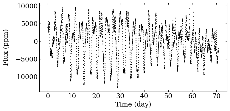
K2: Rotation period analysis

t, s, dt = sp.load_k2_example ()

fig, ax = plt.subplots (1, 1, figsize=(8,4))

ax.scatter (t[s!=0]-t[0], s[s!=0], color='black',
            marker='o', s=1)

ax.set_xlabel ('Time (day)')
ax.set_ylabel ('Flux (ppm)')

fig.tight_layout ()

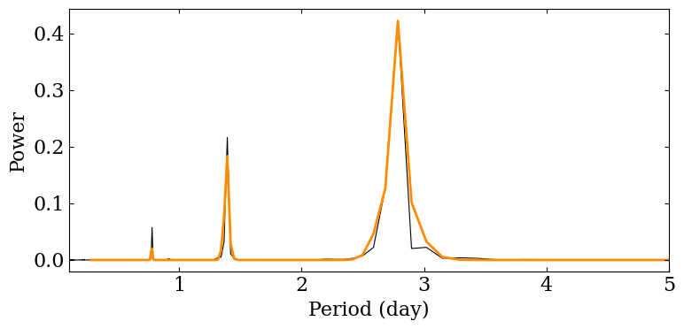
As we want to recover rotation periods below 45 days, we only consider the section of the periodogram verifying \(P < P_\mathrm{cutoff} = 45\) days.

pcutoff = 45

As a preprocessing step, we compute the Lomb-Scargle periodogram (in the SAS framework, it will be directyly provided by MSAP1).

p_ps, ps_object = sp.compute_lomb_scargle (t, s)
ls = ps_object.power_standard_norm

Now we perform the periodogram analysis.

cond = p_ps < pcutoff
prot, e_p, E_p, param, h_ps = sp.compute_prot_err_gaussian_fit_chi2_distribution (p_ps[cond], ls[cond], n_profile=20,
                                                                                     threshold=0.1, plot_procedure=False,
                                                                                     verbose=False)
sp.plot_ls (p_ps, ls, filename='figures/fourier_k2.png', param_profile=param,
               logscale=False, xlim=(0.1, 5))
IDP_123_PROT_FOURIER = sp.prepare_idp_fourier (param, h_ps, ls.size,
                                                  pcutoff=pcutoff, pthresh=None,
                                                  fapcutoff=1e-6)

df = pd.DataFrame (data=IDP_123_PROT_FOURIER)
df

	0	1	2	3	4
0	2.759429	0.036004	0.036968	0.422299	1.000000e-16
1	1.393418	0.013796	0.014075	0.216592	1.000000e-16
2	0.775871	0.007650	0.007804	0.057243	1.000000e-16

df.to_latex (buf='data_products/idp_123_prot_fourier_k2_211015853.tex',
             formatters=['{:.2f}'.format, '{:.2f}'.format, '{:.2f}'.format,
                         '{:.2f}'.format, '{:.0e}'.format],
             index=False, header=False)
np.savetxt ('data_products/IDP_123_PROT_FOURIER_K2.dat',
             IDP_123_PROT_FOURIER)

This time, we are interested in recovering long term modulations. We consider the section of the periodogram verifying \(P > P_\mathrm{tresh} = 90\) days.

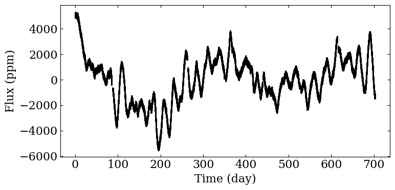
PLATO: Rotation period analysis

filename = sp.get_target_filename (plato_sim_dataset, '040', filetype='csv')
t, s, dt = sp.load_resource (filename)

fig, ax = plt.subplots (1, 1, figsize=(8,4))

ax.scatter (t[s!=0]-t[0], s[s!=0], color='black',
            marker='o', s=1)

ax.set_xlabel ('Time (day)')
ax.set_ylabel ('Flux (ppm)')

fig.tight_layout ()

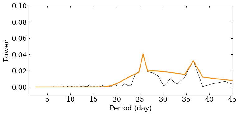
As we want to recover rotation periods below 45 days, we only consider the section of the periodogram verifying \(P < P_\mathrm{cutoff} = 45\) days.

pcutoff = 45

As a preprocessing step, we compute the Lomb-Scargle periodogram (in the SAS framework, it will be directyly provided by MSAP1).

p_ps, ps_object = sp.compute_lomb_scargle (t, s)
ls = ps_object.power_standard_norm

Now we perform the periodogram analysis.

cond = p_ps < pcutoff
prot, e_p, E_p, param, h_ps = sp.compute_prot_err_gaussian_fit_chi2_distribution (p_ps[cond], ls[cond], n_profile=20,
                                                                                     threshold=0.1,
                                                                                     verbose=False)
sp.plot_ls (p_ps, ls, filename='figures/fourier_plato_short.png', param_profile=param,
               logscale=False, xlim=(1, pcutoff), ylim=(-0.01, 0.1))
IDP_123_PROT_FOURIER = sp.prepare_idp_fourier (param, h_ps, ls.size,
                                                  pcutoff=pcutoff, pthresh=None,
                                                  fapcutoff=1e-6)
df = pd.DataFrame (data=IDP_123_PROT_FOURIER)
df

	0	1	2	3	4
0	25.969122	5.252268	8.819944	0.041200	1.000000e-16
1	36.172726	9.338396	19.307071	0.032378	1.000000e-16

df.to_latex (buf='data_products/idp_123_prot_fourier_plato_040.tex',
             formatters=['{:.2f}'.format, '{:.2f}'.format, '{:.2f}'.format,
                         '{:.2f}'.format, '{:.0e}'.format],
             index=False, header=False)
np.savetxt ('data_products/IDP_123_PROT_FOURIER_PLATO.dat',
             IDP_123_PROT_FOURIER)

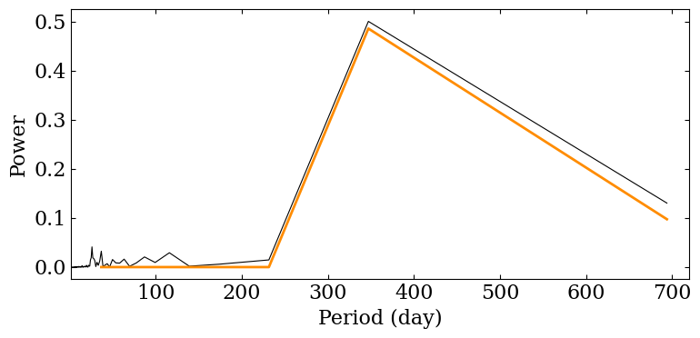
PLATO: Long term modulation analysis

This time, we are interested in recovering long term modulations. We consider the section of the periodogram verifying \(P > P_\mathrm{tresh} = 90\) days.

pthresh = 90

As a preprocessing step, we compute the Lomb-Scargle periodogram (in the SAS framework, it will be directyly provided by MSAP1).

p_ps, ps_object = sp.compute_lomb_scargle (t, s)
ls = ps_object.power_standard_norm

Now we perform the periodogram analysis.

plongterm, e_p, E_p, param, h_ps = sp.compute_prot_err_gaussian_fit_chi2_distribution (p_ps[p_ps>pthresh], ls[p_ps>pthresh],
                                                                                          n_profile=5, threshold=0.1, verbose=False)
fig = sp.plot_ls (p_ps, ls, filename='figures/fourier_plato_long.png', param_profile=param,
                    logscale=False, xlim=(1,8*pthresh))
IDP_123_LONGTERM_MODULATION_FOURIER = sp.prepare_idp_fourier (param, h_ps, ls.size,
                                                                 pcutoff=None, pthresh=pthresh,
                                                                 fapcutoff=1e-6)
df = pd.DataFrame (data=IDP_123_LONGTERM_MODULATION_FOURIER)
df

	0	1	2	3	4
0	347.125305	31.560819	38.575413	0.500829	1.000000e-16
1	701.007116	64.295915	78.739851	0.130459	1.000000e-16

df.to_latex (buf='data_products/idp_123_longterm_modulation_fourier_plato_040.tex',
             formatters=['{:.2f}'.format, '{:.2f}'.format, '{:.2f}'.format,
                         '{:.2f}'.format, '{:.0e}'.format],
             index=False, header=False)
np.savetxt ('data_products/IDP_123_LONGTERM_MODULATION_FOURIER_PLATO.dat',
             IDP_123_LONGTERM_MODULATION_FOURIER)