Time series analysis (MSAP4-02)

import matplotlib.pyplot as plt
import numpy as np
import pandas as pd

import star_privateer as sp
import plato_msap4_demonstrator_datasets.plato_sim_dataset as plato_sim_dataset

K2: Preprocessing

This first part include preprocessing tasks that are not actually included in MSAP4-02 but are useful for the subsequent analysis.

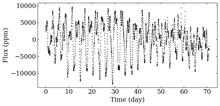
t, s0, dt = sp.load_k2_example ()

fig, ax = plt.subplots (1, 1, figsize=(8,4))

ax.scatter (t[s0!=0]-t[0], s0[s0!=0], color='black',
            marker='o', s=1)

ax.set_xlabel ('Time (day)')
ax.set_ylabel ('Flux (ppm)')

fig.tight_layout ()

plt.savefig ('figures/k2_lc.png', dpi=300)

pcutoff = 60
pthresh = 60

K2: Rotation period analysis

In the next step, we compute the ACF and we analyse the characteristic periodicities obtained from the function, considering only periods below \(P_\mathrm{cutoff}\).

p_acf, acf = sp.compute_acf (s0, dt, normalise=True,
                            use_scipy_correlate=True, verbose=True)
_, _, _, _, prots, hacf, gacf = sp.find_period_acf (p_acf, acf, pcutoff=pcutoff)
fig = sp.plot_acf (p_acf, acf, prot=prots, filename='figures/acf_k2.png')

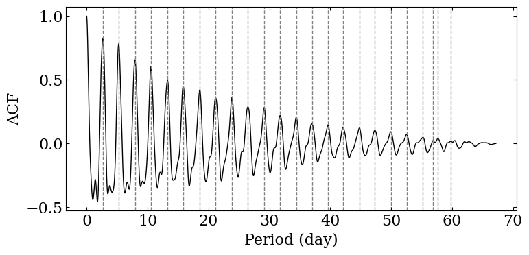
We can take a look at the values we have extracted from the ACF. Most often, the rotation period can be linked to the first value of the prots array.

prots[0], hacf[0], gacf[0]

(2.6765510971308686, 1.219105626528322, 0.8085280511689089)

Finally we create the intermediate data product.

IDP_SAS_ACF_FILT_TIMESERIES = np.c_[p_acf, acf]
IDP_SAS_PROT_TIMESERIES = np.c_[prots, np.full (prots.size, -1), np.full (prots.size, -1),
                                hacf, gacf, np.arange (prots.size)+1]
np.savetxt ('data_products/IDP_SAS_PROT_TIMESERIES_K2.dat',
            IDP_SAS_PROT_TIMESERIES)
np.savetxt ('data_products/IDP_SAS_ACF_FILT_TIMESERIES_K2.dat',
            IDP_SAS_ACF_FILT_TIMESERIES)
df = pd.DataFrame (data=IDP_SAS_PROT_TIMESERIES)
df

	0	1	2	3	4	5
0	2.676551	-1.0	-1.0	1.219106	0.808528	1.0
1	5.271375	-1.0	-1.0	1.142988	0.761694	2.0
2	7.947927	-1.0	-1.0	0.984593	0.642715	3.0
3	10.583614	-1.0	-1.0	0.910175	0.586043	4.0
4	13.280597	-1.0	-1.0	0.746789	0.483461	5.0
5	15.875421	-1.0	-1.0	0.743666	0.437643	6.0
6	18.592836	-1.0	-1.0	0.717921	0.408310	7.0
7	21.187660	-1.0	-1.0	0.642279	0.351740	8.0
8	23.884643	-1.0	-1.0	0.621054	0.350691	9.0
9	26.499899	-1.0	-1.0	0.533378	0.282954	10.0
10	29.156018	-1.0	-1.0	0.508112	0.272964	11.0
11	31.791706	-1.0	-1.0	0.426513	0.215709	12.0
12	34.427394	-1.0	-1.0	0.379729	0.199663	13.0
13	36.981355	-1.0	-1.0	0.304468	0.152380	14.0
14	39.637474	-1.0	-1.0	0.267633	0.141080	15.0
15	42.109708	-1.0	-1.0	0.232925	0.122093	16.0
16	44.786260	-1.0	-1.0	0.219537	0.117616	17.0
17	47.340221	-1.0	-1.0	0.192786	0.100213	18.0
18	49.955477	-1.0	-1.0	0.178725	0.089382	19.0
19	52.550301	-1.0	-1.0	0.154197	0.068293	20.0
20	55.226852	-1.0	-1.0	0.123732	0.046698	21.0
21	56.902250	-1.0	-1.0	0.051635	0.020629	22.0
22	57.678655	-1.0	-1.0	0.064155	0.037136	23.0
23	59.783118	-1.0	-1.0	0.040878	0.015503	24.0

df.to_latex (buf='data_products/idp_msap4_02_idp_prot_timeseries.tex',
             formatters=['{:.2f}'.format, '{:.0f}'.format, '{:.0f}'.format,
                         '{:.2f}'.format, '{:.2f}'.format, '{:.0f}'.format,],
             index=False, header=False)

Note that, due to the short length of this light curve, we do not show for this first case the analysis of long term modulations.

PLATO simulation: Preprocessing

This first part include preprocessing tasks that are not actually included in MSAP4-02 but are useful for the subsequent analysis.

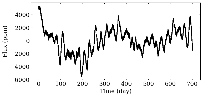
filename = sp.get_target_filename (plato_sim_dataset, '040', filetype='csv')
t, s0, dt = sp.load_resource (filename)

fig, ax = plt.subplots (1, 1, figsize=(8,4))

ax.scatter (t[s0!=0]-t[0], s0[s0!=0], color='black',
            marker='o', s=1)

ax.set_xlabel ('Time (day)')
ax.set_ylabel ('Flux (ppm)')

fig.tight_layout ()


plt.savefig ('figures/plato_lc.png', dpi=300)

s = sp.preprocess (t, s0, cut=60)
pcutoff = 60
pthresh = 60

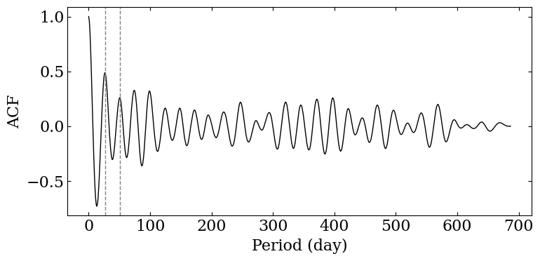
PLATO simulation: Rotation period analysis

This first part include preprocessing task that are not actually included in MSAP4-02 but are useful for the subsequent analysis.

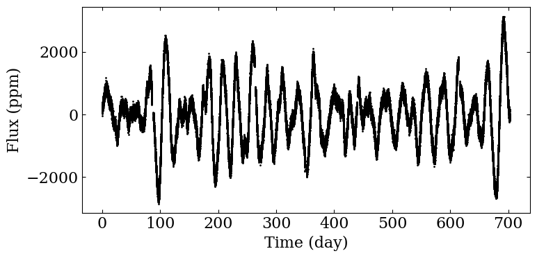
fig, ax = plt.subplots (1, 1, figsize=(8,4))

ax.scatter (t[s!=0]-t[0], s[s!=0], color='black',
            marker='o', s=1)

ax.set_xlabel ('Time (day)')
ax.set_ylabel ('Flux (ppm)')

fig.tight_layout ()

plt.savefig ('figures/plato_lc_filtered.png', dpi=300)

p_acf, acf = sp.compute_acf (s, dt, normalise=True, use_scipy_correlate=True)
_, _, _, _, prots, hacf, gacf = sp.find_period_acf (p_acf, acf, pcutoff=pcutoff)
fig = sp.plot_acf (p_acf, acf, prot=prots, filename='figures/acf_plato_short.png')

IDP_SAS_ACF_FILT_TIMESERIES = np.c_[p_acf, acf]
IDP_SAS_PROT_TIMESERIES = np.c_[prots, np.full (prots.size, -1), np.full (prots.size, -1),
                                hacf, gacf, np.arange (prots.size)+1]
np.savetxt ('data_products/IDP_SAS_PROT_TIMESERIES_PLATO.dat',
            IDP_SAS_PROT_TIMESERIES)
np.savetxt ('data_products/IDP_SAS_ACF_FILT_TIMESERIES_PLATO.dat',
            IDP_SAS_ACF_FILT_TIMESERIES)

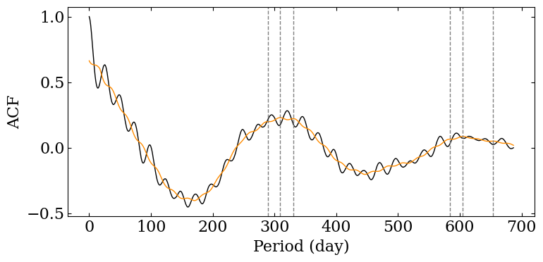
PLATO simulation: Long term modulation analysis

This time, we do not consider filtered out the data in order to consider long term modulations. We put a period threshold at 60 days to consider only long period in the postprocessing of our analysis. In the figure below, note that a Gaussian smoothing window is applied before looking for local maxima, shown in orange in the figure below.

p_acf, acf = sp.compute_acf (s0, dt, normalise=True, pthresh=pthresh,
                            use_scipy_correlate=True, verbose=True)
(_, hacf, gacf, _,
pmods, hacf, gacf, acf_smooth) = sp.find_period_acf (p_acf, acf, pthresh=pthresh,
                                                     return_smoothed_acf=True)
fig = sp.plot_acf (p_acf, acf, prot=pmods,
                   acf_additional=acf_smooth,
                   color_additional="darkorange",
                   filename="figures/acf_plato_long.png")

IDP_SAS_ACF_TIMESERIES = np.c_[p_acf, acf]
IDP_SAS_LONGTERM_MODULATION_TIMESERIES = np.c_[pmods, np.full (pmods.size, -1), np.full (pmods.size, -1),
                                                                hacf, gacf, np.arange (pmods.size)+1]
np.savetxt ('data_products/IDP_SAS_LONGTERM_MODULATION_TIMESERIES_PLATO.dat',
            IDP_SAS_PROT_TIMESERIES)
np.savetxt ('data_products/IDP_SAS_ACF_TIMESERIES_PLATO.dat',
            IDP_SAS_ACF_TIMESERIES)
df = pd.DataFrame (data=IDP_SAS_LONGTERM_MODULATION_TIMESERIES)
df

	0	1	2	3	4	5
0	289.505092	-1.0	-1.0	0.301008	0.199352	1.0
1	309.199410	-1.0	-1.0	0.023280	0.229724	2.0
2	330.483996	-1.0	-1.0	0.200066	0.222273	3.0
3	584.308760	-1.0	-1.0	0.092116	0.065606	4.0
4	604.933628	-1.0	-1.0	0.029614	0.086868	5.0
5	653.718038	-1.0	-1.0	0.009202	0.050910	6.0

df.to_latex (buf='data_products/idp_msap4_02_idp_longterm_modulation_timeseries.tex',
             formatters=['{:.2f}'.format, '{:.0f}'.format, '{:.0f}'.format,
                         '{:.2f}'.format, '{:.2f}'.format, '{:.0f}'.format,],
             index=False, header=False)