Composite spectrum (CS), ROOSTER, and Sph index (MSAP4-03)#
In this notebook, we follow the flowchart defined for the PLATO MSAP4-03 submodule to show how the composite spectrum and the \(S_\mathrm{ph}\) time series are computed. The final rotation period for the star is also computed through the random forest classifier analysis performed by the ROOSTER methodology.
import matplotlib.pyplot as plt
import numpy as np
import pandas as pd
import star_privateer as sp
Preprocessing#
We start by loading our usual K2 light curve (EPIC 211015853) and the intermediate data products we require from MSAP4-01 and 02. We also recompute the Lomb-Scargle periodogram as we need it for the composite spectrum.
t, s, dt = sp.load_k2_example ()
IDP_SAS_PROT_FOURIER = np.loadtxt ('data_products/IDP_SAS_PROT_FOURIER_K2.dat')
IDP_SAS_PROT_TIMESERIES = np.loadtxt ('data_products/IDP_SAS_PROT_TIMESERIES_K2.dat')
IDP_SAS_ACF_FILT_TIMESERIES = np.loadtxt ('data_products/IDP_SAS_ACF_FILT_TIMESERIES_K2.dat')
p_ps, ls = sp.compute_lomb_scargle (t, s)
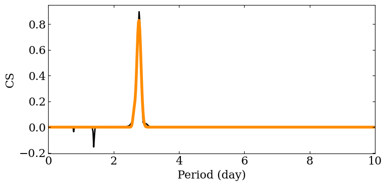
Computing the CS#
The ACF is renormalised by its value at the main periodicity.
prot_acf = IDP_SAS_PROT_TIMESERIES[0,0]/IDP_SAS_PROT_TIMESERIES[0,5]
p_acf, acf = IDP_SAS_ACF_FILT_TIMESERIES[:,0], IDP_SAS_ACF_FILT_TIMESERIES[:,1]
index_prot_acf = np.where (prot_acf==p_acf)[0][0]
cs = sp.compute_cs (ls, acf, p_acf=p_acf, p_ps=p_ps,
                       index_prot_acf=index_prot_acf)
_, hcs = sp.find_prot_cs (p_acf, cs)
(prot_cs, E_prot_cs,
 param_gauss_cs) = sp.compute_prot_err_gaussian_fit (p_acf, cs, verbose=False,
                                                  n_profile=5, threshold=0.1)
fig = sp.plot_cs (p_acf, cs, ax=None, figsize=(8, 4),
                    lw=2, filename='figures/cs_k2.png', dpi=300,
                    param_gauss=param_gauss_cs,
                    xlim=(0, 10))
ROOSTER analysis#
Before using ROOSTER, we must gather the set of parameter it needs for the analysis. The candidate \(S_\mathrm{ph}\) mean values for each possible periods are among this set.
IDP_SAS_PROT_FOURIER.shape
(3, 5)
(prot_ps, e_prot_ps, E_prot_ps,
 h_ps, fa_prob_ps) = (IDP_SAS_PROT_FOURIER[0,0],
                      IDP_SAS_PROT_FOURIER[0,1],
                      IDP_SAS_PROT_FOURIER[0,2],
                      IDP_SAS_PROT_FOURIER[0,3],
                      IDP_SAS_PROT_FOURIER[0,4])
(prot_acf, e_prot_acf, E_prot_acf,
 hacf, gacf) = (IDP_SAS_PROT_TIMESERIES[0,0],
                IDP_SAS_PROT_TIMESERIES[0,1],
                IDP_SAS_PROT_TIMESERIES[0,2],
                IDP_SAS_PROT_TIMESERIES[0,3],
                IDP_SAS_PROT_TIMESERIES[0,4])
sph_ps = sp.compute_sph (t, s, prot_ps)
sph_acf = sp.compute_sph (t, s, prot_acf)
sph_cs = sp.compute_sph (t, s, prot_cs)
features = np.array ([prot_ps, prot_acf, prot_cs,
                     e_prot_ps, E_prot_ps,
                     e_prot_acf, E_prot_acf,
                     E_prot_cs, E_prot_cs,
                     sph_ps, sph_acf, sph_cs,
                     h_ps, fa_prob_ps, hacf, gacf, hcs])
feature_names = np.array(['prot_ps', 'prot_acf', 'prot_cs',
                         'e_prot_ps', 'E_prot_ps',
                         'e_prot_acf', 'E_prot_acf',
                         'e_prot_cs', 'E_prot_cs',
                         'sph_ps', 'sph_acf', 'sph_cs',
                         'h_ps', 'fa_prob_ps',
                         'hacf', 'gacf', 'hcs'])
df = pd.DataFrame (columns=feature_names, index=[211015853],
                   data=features.reshape (-1, features.size))
df
| prot_ps | prot_acf | prot_cs | e_prot_ps | E_prot_ps | e_prot_acf | E_prot_acf | e_prot_cs | E_prot_cs | sph_ps | sph_acf | sph_cs | h_ps | fa_prob_ps | hacf | gacf | hcs | |
|---|---|---|---|---|---|---|---|---|---|---|---|---|---|---|---|---|---|
| 211015853 | 2.786835 | 2.676551 | 2.772695 | 0.027592 | 0.02815 | -1.0 | -1.0 | 0.090589 | 0.090589 | 4594.719727 | 4672.765625 | 4606.483398 | 18241.430962 | 1.000000e-16 | 1.219106 | 0.808528 | 0.895935 |
We create the data structure that ROOSTER will need.
(target_id, p_candidates,
 e_p_candidates, E_p_candidates,
 features, feature_names) = sp.create_rooster_feature_inputs (df, return_err=True)
p_candidates
array([[2.78683526, 2.6765511 , 2.77269456]])
Now, we load and use the ROOSTER object.
chicken = sp.load_rooster_instance (filename='rooster_instances/rooster_tutorial')
rotation_score, prot, e_p, E_p = chicken.analyseSet (features, p_candidates, e_p_err=e_p_candidates,
                                                     E_p_err=E_p_candidates, feature_names=feature_names)
rotation_score, prot, e_p, E_p
(array([0.63]), array([2.78683526]), array([0.02759243]), array([0.02814985]))
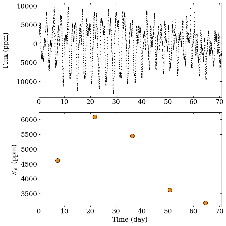
Computing \(S_\mathrm{ph}\) time series#
Now that we have the final value of the rotation period, we can correctly compute the \(S_\mathrm{ph}\) time series.
_, t_sph, sph_series = sp.compute_sph (t, s, prot,
                                          return_timeseries=True)
We show below the \(S_\mathrm{ph}\) evolution along time compared with the time series flux evolution.
fig, (ax1, ax2) = plt.subplots (2, 1, figsize=(8,8))

ax1.scatter (t - t[0], s, marker='o', facecolor='black', s=1)
ax2.scatter (t_sph - t[0], sph_series, marker='o', s=100,
            facecolor='darkorange', edgecolor='black')

ax1.set_ylabel (r'Flux (ppm)')
ax2.set_xlabel ('Time (day)')
ax2.set_ylabel (r'$S_\mathrm{ph}$ (ppm)')

ax1.set_xlim (0, t[-1]-t[0])
ax2.set_xlim (0, t[-1]-t[0])

fig.tight_layout ()

plt.savefig ('figures/sph_k2.png', dpi=300)
Computing the Rossby number#
It is now possible to compute an estimate of the fluid Rossby number from the rotation period and the effective temperature. Here, we use the \(T_\mathrm{eff} = 5888\) value from the GAIA DR3 catalog.
teff = 5888
ro, flag = sp.compute_rossby (prot[0], teff)
ro, flag
(0.11723307180128995, 5)
Differential rotation candidates validation#
We now use IDP_SAS_PROT_FOURIER to validate the possible differential rotation candidates.
dr, e_dr, E_dr, shear = sp.compute_delta_prot (prot[0], IDP_SAS_PROT_FOURIER[1:,0],
                                           IDP_SAS_PROT_FOURIER[1:,1],
                                           IDP_SAS_PROT_FOURIER[1:,2],
                                           delta_min=1/3, delta_max=5/3,
                                           tol_harmonic=0.05)
dr, e_dr, E_dr, shear
(-1, -1, -1, -1)
Building the data products#
Finally, we build the data products from the previous computations.
IDP_SAS_S_PHOTO_INDEX = np.c_[t_sph, sph_series]
IDP_SAS_PROT_NOSPOT = np.array ([prot[0], e_p[0], E_p[0],
                                 rotation_score[0], ro,
                                 np.mean (sph_series), np.std (sph_series)])
IDP_SAS_DELTA_PROT_NOSPOT = np.c_[dr, e_dr, E_dr, shear]
np.savetxt ('data_products/IDP_SAS_S_PHOTO_INDEX_K2.dat', IDP_SAS_S_PHOTO_INDEX)
np.savetxt ('data_products/IDP_SAS_PROT_NOSPOT_K2.dat', IDP_SAS_PROT_NOSPOT)
np.savetxt ('data_products/IDP_SAS_DELTA_PROT_K2.dat', IDP_SAS_DELTA_PROT_NOSPOT)