Fourier analysis (MSAP4-01A)#
import star_privateer as sp
import plato_msap4_demonstrator_datasets.plato_sim_dataset as plato_sim_dataset
import numpy as np
import matplotlib.pyplot as plt
import pandas as pd
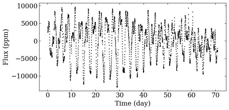
K2: Rotation period analysis#
t, s, dt = sp.load_k2_example ()
fig, ax = plt.subplots (1, 1, figsize=(8,4))

ax.scatter (t[s!=0]-t[0], s[s!=0], color='black',
            marker='o', s=1)

ax.set_xlabel ('Time (day)')
ax.set_ylabel ('Flux (ppm)')

fig.tight_layout ()
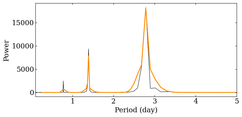
As we want to recover rotation periods below 45 days, we only consider the section of the periodogram verifying \(P < P_\mathrm{cutoff} = 60\) days.
pcutoff = 60
As a preprocessing step, we compute the Lomb-Scargle periodogram (in the SAS framework, it will be directyly provided by MSAP1).
p_ps, ls = sp.compute_lomb_scargle (t, s)
Now we perform the periodogram analysis.
cond = p_ps < pcutoff
(prot, e_p, E_p,
 _, param, h_ps) = sp.compute_prot_err_gaussian_fit_chi2_distribution (p_ps[cond], ls[cond], n_profile=20,
                                                                       threshold=0.1, plot_procedure=False,
                                                                       verbose=False)
fig= sp.plot_ls (p_ps, ls, filename='figures/fourier_k2.png', param_profile=param,
                 logscale=False, xlim=(0.1, 5))
IDP_SAS_PROT_FOURIER = sp.prepare_idp_fourier (param, h_ps, ls.size,
                                              pcutoff=pcutoff, pthresh=None,
                                              pfacutoff=1e-6)

df = pd.DataFrame (data=IDP_SAS_PROT_FOURIER)
df
| 0 | 1 | 2 | 3 | 4 | |
|---|---|---|---|---|---|
| 0 | 2.786835 | 0.027592 | 0.028150 | 18241.430962 | 1.000000e-16 |
| 1 | 1.393417 | 0.013796 | 0.014075 | 9355.805501 | 1.000000e-16 |
| 2 | 0.786985 | 0.056182 | 0.065540 | 2472.622236 | 1.000000e-16 |
df.to_latex (buf='data_products/idp_sas_prot_fourier_k2_211015853.tex',
             formatters=['{:.2f}'.format, '{:.2f}'.format, '{:.2f}'.format,
                         '{:.2f}'.format, '{:.0e}'.format],
             index=False, header=False)
np.savetxt ('data_products/IDP_SAS_PROT_FOURIER_K2.dat',
             IDP_SAS_PROT_FOURIER)
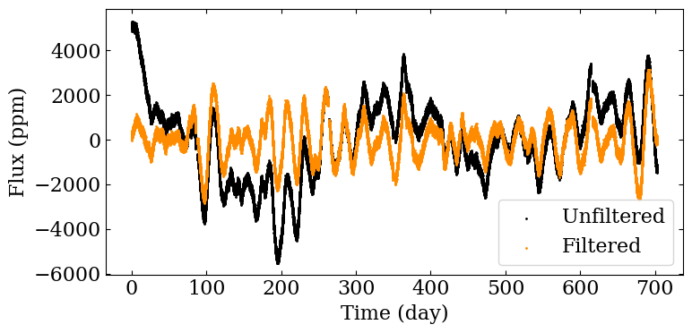
PLATO: Rotation period analysis#
The PLATO simulation below encompasses both rotational modulation and low-frequency modulations due to activity. In order to analyse the rotational signal, we first filter out frequencies above 60 days (in PLATO, this will be done outside MSAP4).
filename = sp.get_target_filename (plato_sim_dataset, '040', filetype='csv')
t, s, dt = sp.load_resource (filename)
s_filtered = sp.preprocess (t, s, cut=60)
fig, ax = plt.subplots (1, 1, figsize=(8,4))

ax.scatter (t[s!=0]-t[0], s[s!=0], color='black',
            marker='o', s=1, label="Unfiltered")
ax.scatter (t[s!=0]-t[0], s_filtered[s_filtered!=0], color='darkorange',
            marker='o', s=1, label="Filtered")

ax.set_xlabel ('Time (day)')
ax.set_ylabel ('Flux (ppm)')

ax.legend ()

fig.tight_layout ()
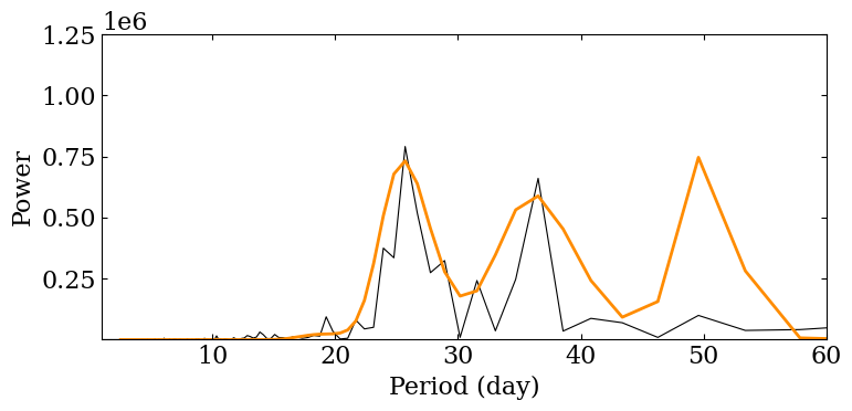
As we want to recover rotation periods below 60 days, we only consider the section of the periodogram verifying \(P < P_\mathrm{cutoff} = 60\) days.
pcutoff = 60
As a preprocessing step, we compute the Lomb-Scargle periodogram (in the SAS framework, it will be directyly provided by MSAP1).
p_ps, ls = sp.compute_lomb_scargle (t, s_filtered)
Now we perform the periodogram analysis.
cond = p_ps < pcutoff
(prot, e_p, E_p,
 _, param, h_ps) = sp.compute_prot_err_gaussian_fit_chi2_distribution (p_ps[cond],
                                                                       ls[cond],
                                                                       n_profile=20,
                                                                       threshold=0.1,
                                                                       verbose=False)
sp.plot_ls (p_ps, ls, filename='figures/fourier_plato_short.png', param_profile=param,
            logscale=False, xlim=(1, pcutoff),
            ylim=(1e-3, 1.25e6),
            )
IDP_SAS_PROT_FOURIER = sp.prepare_idp_fourier (param, h_ps, ls.size,
                                                  pcutoff=pcutoff, pthresh=None,
                                                  pfacutoff=1e-6)
df = pd.DataFrame (data=IDP_SAS_PROT_FOURIER)
df
| 0 | 1 | 2 | 3 | 4 | |
|---|---|---|---|---|---|
| 0 | 25.969122 | 2.720310 | 3.441268 | 791101.027115 | 1.000000e-16 |
| 1 | 36.172726 | 3.871280 | 4.925569 | 660816.783569 | 1.000000e-16 |
| 2 | 50.083306 | 2.931017 | 3.319557 | 99449.921037 | 1.000000e-16 |
| 3 | 19.091161 | 2.501881 | 3.390534 | 93860.256080 | 1.000000e-16 |
df.to_latex (buf='data_products/idp_sas_prot_fourier_plato_040.tex',
             formatters=['{:.2f}'.format, '{:.2f}'.format, '{:.2f}'.format,
                         '{:.2f}'.format, '{:.0e}'.format],
             index=False, header=False)
np.savetxt ('data_products/IDP_SAS_PROT_FOURIER_PLATO.dat',
             IDP_SAS_PROT_FOURIER)
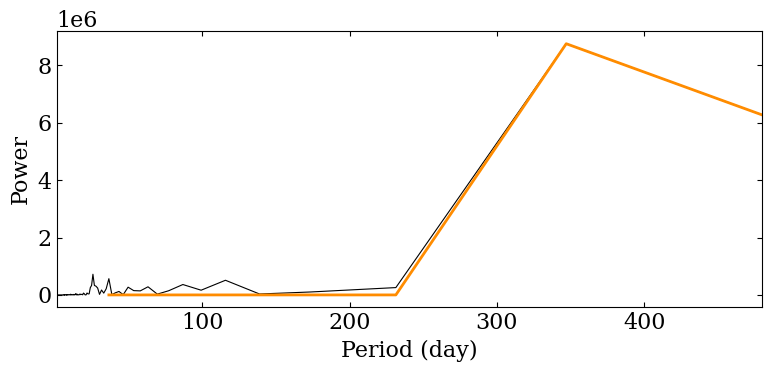
PLATO: Long term modulation analysis#
This time, we are interested in recovering long term modulations. We consider the section of the periodogram verifying \(P > P_\mathrm{tresh} = 60\) days.
pthresh = 60
As a preprocessing step, we compute the Lomb-Scargle periodogram (in the SAS framework, it will be directyly provided by MSAP1).
p_ps, ls = sp.compute_lomb_scargle (t, s)
Now we perform the periodogram analysis.
(plongterm, e_p, E_p,
 _, param, h_ps) = sp.compute_prot_err_gaussian_fit_chi2_distribution (p_ps[p_ps>pthresh],
                                                                       ls[p_ps>pthresh],
                                                                       n_profile=5,
                                                                       threshold=0.1,
                                                                       verbose=False)
fig = sp.plot_ls (p_ps, ls, filename='figures/fourier_plato_long.png', param_profile=param,
                    logscale=False, xlim=(1,8*pthresh))
IDP_SAS_LONGTERM_MODULATION_FOURIER = sp.prepare_idp_fourier (param, h_ps, ls.size,
                                                                 pcutoff=None, pthresh=pthresh,
                                                                 pfacutoff=1e-6)
df = pd.DataFrame (data=IDP_SAS_LONGTERM_MODULATION_FOURIER)
df
| 0 | 1 | 2 | 3 | 4 | |
|---|---|---|---|---|---|
| 0 | 347.077309 | 16.527491 | 18.267227 | 8.754753e+06 | 1.000000e-16 |
| 1 | 694.154619 | 33.054982 | 36.534454 | 2.280495e+06 | 1.000000e-16 |
df.to_latex (buf='data_products/idp_sas_longterm_modulation_fourier_plato_040.tex',
             formatters=['{:.2f}'.format, '{:.2f}'.format, '{:.2f}'.format,
                         '{:.2f}'.format, '{:.0e}'.format],
             index=False, header=False)
np.savetxt ('data_products/IDP_SAS_LONGTERM_MODULATION_FOURIER_PLATO.dat',
             IDP_SAS_LONGTERM_MODULATION_FOURIER)