Fourier analysis (MSAP4-01A)#
import star_privateer as sp
import plato_msap4_demonstrator_datasets.plato_sim_dataset as plato_sim_dataset
import numpy as np
import matplotlib.pyplot as plt
import pandas as pd
sp.__version__
'1.2.0'
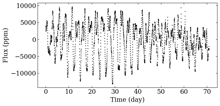
K2: Rotation period analysis#
t, s, dt = sp.load_k2_example ()
fig, ax = plt.subplots (1, 1, figsize=(8,4))

ax.scatter (t[s!=0]-t[0], s[s!=0], color='black',
            marker='o', s=1)

ax.set_xlabel ('Time (day)')
ax.set_ylabel ('Flux (ppm)')

fig.tight_layout ()
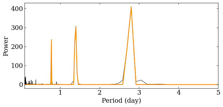
As we want to recover rotation periods below 45 days, we only consider the section of the periodogram verifying \(P < P_\mathrm{cutoff} = 60\) days.
pcutoff = 60
As a preprocessing step, we compute the Lomb-Scargle periodogram (in the SAS framework, it will be directyly provided by MSAP1).
p_ps, ls = sp.compute_lomb_scargle (t, s)
Now we perform the periodogram analysis.
cond = p_ps < pcutoff
(prot, e_p, E_p,
 _, param, h_ps) = sp.compute_prot_err_gaussian_fit_chi2_distribution (p_ps[cond], ls[cond], pfa_threshold=1e-6,
                                                                       plot_procedure=False,
                                                                       verbose=False)
fig= sp.plot_ls (p_ps, ls, filename='figures/fourier_k2.png', param_profile=param,
                 logscale=False, xlim=(0.1, 5))
IDP_SAS_PROT_FOURIER = sp.prepare_idp_fourier (param, h_ps, ls.size,
                                              pcutoff=pcutoff, pthresh=None,
                                              pfacutoff=1e-6)

df = pd.DataFrame (data=IDP_SAS_PROT_FOURIER)
df
| 0 | 1 | 2 | 3 | 4 | |
|---|---|---|---|---|---|
| 0 | 2.800785 | 0.002798 | 0.002804 | 408.999297 | 1.000000e-16 |
| 1 | 1.400584 | 0.001399 | 0.001402 | 307.750010 | 1.000000e-16 |
| 2 | 0.781536 | 0.000781 | 0.000782 | 237.424642 | 1.000000e-16 |
| 3 | 1.371679 | 0.001370 | 0.001373 | 228.878140 | 1.000000e-16 |
| 4 | 2.688480 | 0.002685 | 0.002691 | 179.810535 | 1.000000e-16 |
| 5 | 1.429956 | 0.001428 | 0.001431 | 63.878992 | 1.000000e-16 |
| 6 | 0.127013 | 0.000009 | 0.000009 | 41.450787 | 1.000000e-16 |
df.to_latex (buf='data_products/idp_sas_prot_fourier_k2_211015853.tex',
             formatters=['{:.2f}'.format, '{:.2f}'.format, '{:.2f}'.format,
                         '{:.2f}'.format, '{:.0e}'.format],
             index=False, header=False)
np.savetxt ('data_products/IDP_SAS_PROT_FOURIER_K2.dat',
             IDP_SAS_PROT_FOURIER)
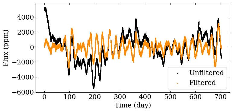
PLATO: Rotation period analysis#
The PLATO simulation below encompasses both rotational modulation and low-frequency modulations due to activity. In order to analyse the rotational signal, we first filter out frequencies above 60 days (in PLATO, this will be done outside MSAP4).
filename = sp.get_target_filename (plato_sim_dataset, '040', filetype='csv')
t, s, dt = sp.load_resource (filename)
s_filtered = sp.preprocess (t, s, cut=60)
fig, ax = plt.subplots (1, 1, figsize=(8,4))

ax.scatter (t[s!=0]-t[0], s[s!=0], color='black',
            marker='o', s=1, label="Unfiltered")
ax.scatter (t[s!=0]-t[0], s_filtered[s_filtered!=0], color='darkorange',
            marker='o', s=1, label="Filtered")

ax.set_xlabel ('Time (day)')
ax.set_ylabel ('Flux (ppm)')

ax.legend ()

fig.tight_layout ()
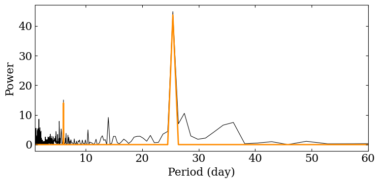
As we want to recover rotation periods below 60 days, we only consider the section of the periodogram verifying \(P < P_\mathrm{cutoff} = 60\) days.
pcutoff = 60
As a preprocessing step, we compute the Lomb-Scargle periodogram (in the SAS framework, it will be directyly provided by MSAP1).
p_ps, ls = sp.compute_lomb_scargle (t, s_filtered)
Now we perform the periodogram analysis.
cond = p_ps < pcutoff
(prot, e_p, E_p,
 _, param, h_ps) = sp.compute_prot_err_gaussian_fit_chi2_distribution (p_ps[cond],
                                                                       ls[cond],
                                                                       pfa_threshold=1e-6,
                                                                       verbose=False)
sp.plot_ls (p_ps, ls, filename='figures/fourier_plato_short.png', param_profile=param,
            logscale=False, xlim=(1, pcutoff),
            )
IDP_SAS_PROT_FOURIER = sp.prepare_idp_fourier (param, h_ps, ls.size,
                                              pcutoff=pcutoff, pthresh=None,
                                              pfacutoff=1e-6)
df = pd.DataFrame (data=IDP_SAS_PROT_FOURIER)
df
| 0 | 1 | 2 | 3 | 4 | |
|---|---|---|---|---|---|
| 0 | 25.433099 | 0.025403 | 0.025454 | 44.875420 | 1.000000e-16 |
| 1 | 6.076207 | 0.006068 | 0.006080 | 15.077311 | 2.831438e-07 |
df.to_latex (buf='data_products/idp_sas_prot_fourier_plato_040.tex',
             formatters=['{:.2f}'.format, '{:.2f}'.format, '{:.2f}'.format,
                         '{:.2f}'.format, '{:.0e}'.format],
             index=False, header=False)
np.savetxt ('data_products/IDP_SAS_PROT_FOURIER_PLATO.dat',
             IDP_SAS_PROT_FOURIER)
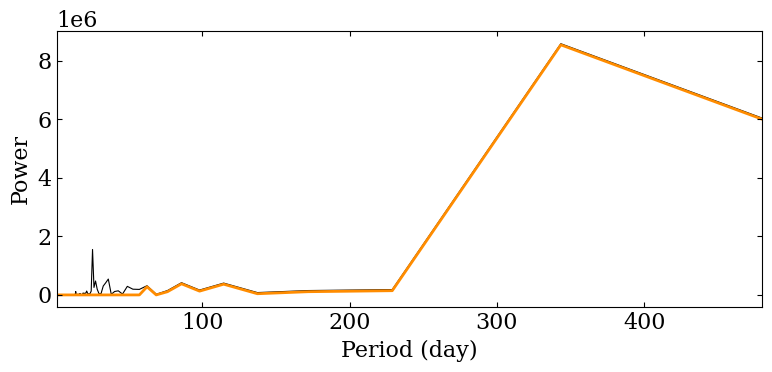
PLATO: Long term modulation analysis#
This time, we are interested in recovering long term modulations. We consider the section of the periodogram verifying \(P > P_\mathrm{tresh} = 60\) days.
pthresh = 60
As a preprocessing step, we compute the Lomb-Scargle periodogram (in the SAS framework, it will be directyly provided by MSAP1).
p_ps, ls = sp.compute_lomb_scargle (t, s, normalisation="snr_flat")
Now we perform the periodogram analysis.
(plongterm, e_p, E_p,
 _, param, h_ps) = sp.compute_prot_err_gaussian_fit_chi2_distribution (p_ps[p_ps>pthresh],
                                                                       ls[p_ps>pthresh],
                                                                       pfa_threshold=1e-6,
                                                                       verbose=False)
fig = sp.plot_ls (p_ps, ls, filename='figures/fourier_plato_long.png', param_profile=param,
                    logscale=False, xlim=(1,8*pthresh))
IDP_SAS_LONGTERM_MODULATION_FOURIER = sp.prepare_idp_fourier (param, h_ps, ls.size,
                                                              pcutoff=None, pthresh=pthresh,
                                                              pfacutoff=1e-6)
df = pd.DataFrame (data=IDP_SAS_LONGTERM_MODULATION_FOURIER)
df
| 0 | 1 | 2 | 3 | 4 | |
|---|---|---|---|---|---|
| 0 | 343.497833 | 0.343238 | 0.343925 | 8.576472e+06 | 1.000000e-16 |
| 1 | 685.994492 | 0.684484 | 0.685852 | 2.198985e+06 | 1.000000e-16 |
| 2 | 85.690887 | 0.085443 | 0.085613 | 4.172111e+05 | 1.000000e-16 |
| 3 | 114.308839 | 0.114031 | 0.114259 | 4.035625e+05 | 1.000000e-16 |
| 4 | 62.343966 | 0.062187 | 0.062311 | 3.141029e+05 | 1.000000e-16 |
| 5 | 228.516929 | 0.227862 | 0.228317 | 1.820337e+05 | 1.000000e-16 |
| 6 | 97.934998 | 0.097654 | 0.097849 | 1.662900e+05 | 1.000000e-16 |
| 7 | 171.403827 | 0.170925 | 0.171267 | 1.490459e+05 | 1.000000e-16 |
| 8 | 76.173568 | 0.075956 | 0.076108 | 1.486087e+05 | 1.000000e-16 |
| 9 | 137.128087 | 0.136749 | 0.137022 | 8.018874e+04 | 1.000000e-16 |
df.to_latex (buf='data_products/idp_sas_longterm_modulation_fourier_plato_040.tex',
             formatters=['{:.2f}'.format, '{:.2f}'.format, '{:.2f}'.format,
                         '{:.2f}'.format, '{:.0e}'.format],
             index=False, header=False)
np.savetxt ('data_products/IDP_SAS_LONGTERM_MODULATION_FOURIER_PLATO.dat',
             IDP_SAS_LONGTERM_MODULATION_FOURIER)