Time series analysis (MSAP4-02)

import matplotlib.pyplot as plt
import numpy as np
import pandas as pd

import star_privateer as sp
import plato_msap4_demonstrator_datasets.plato_sim_dataset as plato_sim_dataset

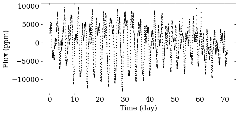
K2: Preprocessing

This first part include preprocessing tasks that are not actually included in MSAP4-02 but are useful for the subsequent analysis.

t, s0, dt = sp.load_k2_example ()

fig, ax = plt.subplots (1, 1, figsize=(8,4))

ax.scatter (t[s0!=0]-t[0], s0[s0!=0], color='black',
            marker='o', s=1)

ax.set_xlabel ('Time (day)')
ax.set_ylabel ('Flux (ppm)')

fig.tight_layout ()

plt.savefig ('figures/k2_lc.png', dpi=300)

pcutoff = 60
pthresh = 60

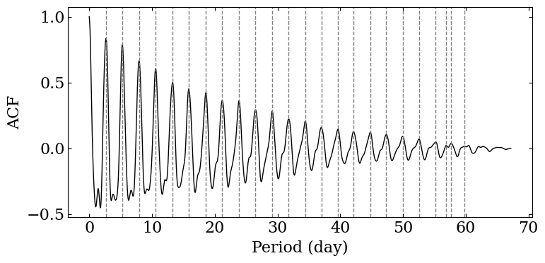
K2: Rotation period analysis

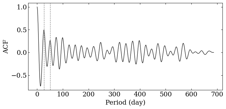
In the next step, we compute the ACF and we analyse the characteristic periodicities obtained from the function, considering only periods below \(P_\mathrm{cutoff}\).

p_acf, acf = sp.compute_acf (s0, dt, normalise=True,
                                use_scipy_correlate=True, smooth=True, verbose=True)
_, _, _, _, prots, hacf, gacf = sp.find_period_acf (p_acf, acf, pcutoff=pcutoff)
fig = sp.plot_acf (p_acf, acf, prot=prots, filename='figures/acf_k2.png')

ACF was smoothed with a period 0.26 days

We can take a look at the values we have extracted from the ACF. Most often, the rotation period can be linked to the first value of the prots array.

prots[0], hacf[0], gacf[0]

(2.6765510971308686, 1.2594916191360066, 0.8353126108493093)

Finally we create the intermediate data product.

IDP_SAS_ACF_FILT_TIMESERIES = np.c_[p_acf, acf]
IDP_SAS_PROT_TIMESERIES = np.c_[prots, np.full (prots.size, -1), np.full (prots.size, -1),
                                hacf, gacf, np.arange (prots.size)+1]
np.savetxt ('data_products/IDP_SAS_PROT_TIMESERIES_K2.dat',
            IDP_SAS_PROT_TIMESERIES)
np.savetxt ('data_products/IDP_SAS_ACF_FILT_TIMESERIES_K2.dat',
            IDP_SAS_ACF_FILT_TIMESERIES)
df = pd.DataFrame (data=IDP_SAS_PROT_TIMESERIES)
df

	0	1	2	3	4	5
0	2.676551	-1.0	-1.0	1.259492	0.835313	1.0
1	5.271375	-1.0	-1.0	1.180853	0.786927	2.0
2	7.947927	-1.0	-1.0	1.017210	0.664006	3.0
3	10.583614	-1.0	-1.0	0.940327	0.605458	4.0
4	13.280597	-1.0	-1.0	0.771528	0.499477	5.0
5	15.875421	-1.0	-1.0	0.768302	0.452141	6.0
6	18.592836	-1.0	-1.0	0.741704	0.421836	7.0
7	21.187660	-1.0	-1.0	0.663556	0.363392	8.0
8	23.884643	-1.0	-1.0	0.641628	0.362309	9.0
9	26.499899	-1.0	-1.0	0.551047	0.292327	10.0
10	29.156018	-1.0	-1.0	0.524945	0.282007	11.0
11	31.791706	-1.0	-1.0	0.440642	0.222855	12.0
12	34.427394	-1.0	-1.0	0.392308	0.206277	13.0
13	36.981355	-1.0	-1.0	0.314554	0.157428	14.0
14	39.637474	-1.0	-1.0	0.276499	0.145753	15.0
15	42.109708	-1.0	-1.0	0.240641	0.126138	16.0
16	44.786260	-1.0	-1.0	0.226810	0.121512	17.0
17	47.340221	-1.0	-1.0	0.199173	0.103533	18.0
18	49.955477	-1.0	-1.0	0.184646	0.092344	19.0
19	52.550301	-1.0	-1.0	0.159305	0.070555	20.0
20	55.226852	-1.0	-1.0	0.127831	0.048245	21.0
21	56.902250	-1.0	-1.0	0.053345	0.021313	22.0
22	57.678655	-1.0	-1.0	0.066281	0.038367	23.0
23	59.783118	-1.0	-1.0	0.042232	0.016017	24.0

df.to_latex (buf='data_products/idp_msap4_02_idp_prot_timeseries.tex',
             formatters=['{:.2f}'.format, '{:.0f}'.format, '{:.0f}'.format,
                         '{:.2f}'.format, '{:.2f}'.format, '{:.0f}'.format,],
             index=False, header=False)

Note that, due to the short length of this light curve, we do not show for this first case the analysis of long term modulations.

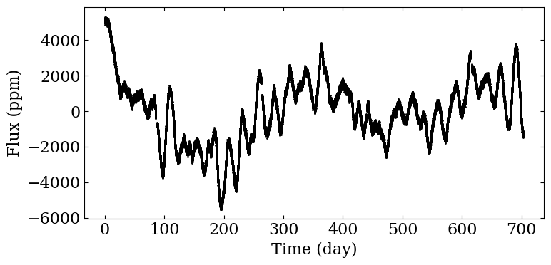
PLATO simulation: Preprocessing

This first part include preprocessing tasks that are not actually included in MSAP4-02 but are useful for the subsequent analysis.

filename = sp.get_target_filename (plato_sim_dataset, '040', filetype='csv')
t, s0, dt = sp.load_resource (filename)

fig, ax = plt.subplots (1, 1, figsize=(8,4))

ax.scatter (t[s0!=0]-t[0], s0[s0!=0], color='black',
            marker='o', s=1)

ax.set_xlabel ('Time (day)')
ax.set_ylabel ('Flux (ppm)')

fig.tight_layout ()


plt.savefig ('figures/plato_lc.png', dpi=300)

s = sp.preprocess (t, s0, cut=60)
pcutoff = 60
pthresh = 60

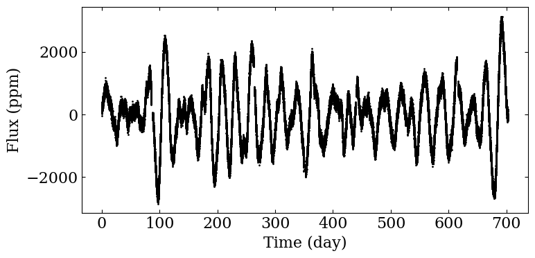
PLATO simulation: Rotation period analysis

This first part include preprocessing task that are not actually included in MSAP4-02 but are useful for the subsequent analysis.

fig, ax = plt.subplots (1, 1, figsize=(8,4))

ax.scatter (t[s!=0]-t[0], s[s!=0], color='black',
            marker='o', s=1)

ax.set_xlabel ('Time (day)')
ax.set_ylabel ('Flux (ppm)')

fig.tight_layout ()

plt.savefig ('figures/plato_lc_filtered.png', dpi=300)

p_acf, acf = sp.compute_acf (s, dt, normalise=True,
                                use_scipy_correlate=True, smooth=True)
_, _, _, _, prots, hacf, gacf = sp.find_period_acf (p_acf, acf, pcutoff=pcutoff)
fig = sp.plot_acf (p_acf, acf, prot=prots, filename='figures/acf_plato_short.png')

IDP_SAS_ACF_FILT_TIMESERIES = np.c_[p_acf, acf]
IDP_SAS_PROT_TIMESERIES = np.c_[prots, np.full (prots.size, -1), np.full (prots.size, -1),
                                hacf, gacf, np.arange (prots.size)+1]
np.savetxt ('data_products/IDP_SAS_PROT_TIMESERIES_PLATO.dat',
            IDP_SAS_PROT_TIMESERIES)
np.savetxt ('data_products/IDP_SAS_ACF_FILT_TIMESERIES_PLATO.dat',
            IDP_SAS_ACF_FILT_TIMESERIES)

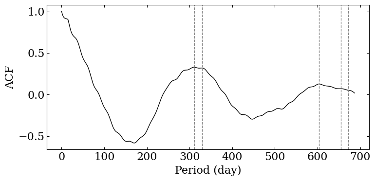
PLATO simulation: Long term modulation analysis

This time, we do not consider filtered out the data in order to consider long term modulations. We put a period threshold at 90 days to consider only long period in the postprocessing of our analysis.

p_acf, acf = sp.compute_acf (s0, dt, normalise=True, pthresh=pthresh, smooth_period=30,
                                use_scipy_correlate=True, smooth=True, verbose=True)
_, hacf, gacf, _, pmods, hacf, gacf = sp.find_period_acf (p_acf, acf, pthresh=pthresh)
fig = sp.plot_acf (p_acf, acf, prot=pmods, filename='figures/acf_plato_long.png')

ACF was smoothed with a period 30.00 days

IDP_SAS_ACF_TIMESERIES = np.c_[p_acf, acf]
IDP_SAS_LONGTERM_MODULATION_TIMESERIES = np.c_[pmods, np.full (pmods.size, -1), np.full (pmods.size, -1),
                                                                hacf, gacf, np.arange (pmods.size)+1]
np.savetxt ('data_products/IDP_SAS_LONGTERM_MODULATION_TIMESERIES_PLATO.dat',
            IDP_SAS_PROT_TIMESERIES)
np.savetxt ('data_products/IDP_SAS_ACF_TIMESERIES_PLATO.dat',
            IDP_SAS_ACF_TIMESERIES)
df = pd.DataFrame (data=IDP_SAS_LONGTERM_MODULATION_TIMESERIES)
df

	0	1	2	3	4	5
0	310.678567	-1.0	-1.0	0.462692	0.329725	1.0
1	328.845118	-1.0	-1.0	0.282649	0.320247	2.0
2	603.628081	-1.0	-1.0	0.180539	0.127609	3.0
3	654.579144	-1.0	-1.0	0.010281	0.070637	4.0
4	671.849867	-1.0	-1.0	-1.000000	0.050842	5.0

df.to_latex (buf='data_products/idp_msap4_02_idp_longterm_modulation_timeseries.tex',
             formatters=['{:.2f}'.format, '{:.0f}'.format, '{:.0f}'.format,
                         '{:.2f}'.format, '{:.2f}'.format, '{:.0f}'.format,],
             index=False, header=False)