Cycle determination (MSAP4-06)#
This notebook provides the test cases described in the MSAP4-06 submodule documentation.
import star_privateer as sp
import numpy as np
import matplotlib.pyplot as plt
Preprocessing#
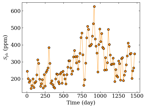
In order to demonstrate the ability of MSAP4-06, we choose KIC~3733735, as its observing time/rotation period ratio is important and will allow us to perform meaningful computation on the \(S_\mathrm{ph}\) time series. We then start by computing this ACF time series, which is normally an IDP input provided by MSAP4-03. We consider the 2.57 days rotation period from Santos et al. (2021).
filename = sp.get_target_filename (sp.timeseries, '003733735')
t, s, dt = sp.load_resource (filename)
pcutoff = (t[-1]-t[0])/2
prot = 2.57
_, t_sph, sph = sp.compute_sph (t, s, prot,
                                          return_timeseries=True)
fig, ax = plt.subplots (1, 1)

ax.plot (t_sph, sph, color='darkorange', zorder=-1)
ax.scatter (t_sph, sph, color='darkorange', edgecolor='black',
            marker='o', s=40)

ax.set_xlabel ('Time (day)')
ax.set_ylabel (r'$S_\mathrm{ph}$ (ppm)')

fig.tight_layout ()

plt.savefig ('figures/kic3733735_sph_timeseries.png', dpi=300)
Computing the ACF and GLS of the ACF time series#
Now that we have our \(S_\mathrm{ph}\) time series, let’s compute its autocorrelation function and analyse it to extract periodicities above \(P_\mathrm{thresh}\).
dt_sph = np.median (np.diff (t_sph))
p_acf_sph, acf_sph = sp.compute_acf (sph - np.mean (sph), dt_sph, normalise=True,
                                        use_scipy_correlate=True, smooth=False)
_, _, _, _, pmods_sph_acf, hacf, gacf = sp.find_period_acf (p_acf_sph, acf_sph, pcutoff=pcutoff)
fig = sp.plot_acf (p_acf_sph, acf_sph, prot=pmods_sph_acf,
                      xlim=(0,750), filename='figures/kic3733735_sph_acf.png')
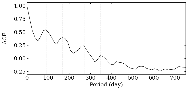
pmods_sph_acf, hacf, gacf
(array([ 89.82634128, 166.82034809, 269.47902383, 346.47303064]),
 array([0.24586367, 0.21436216, 0.22554245, 0.14562127]),
 array([0.54345038, 0.39418935, 0.23732771, 0.0511166 ]))
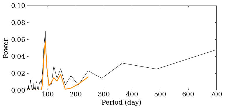
The second step is to compute the Lomb-Scargle periodogram of our \(S_\mathrm{ph}\) time series.
p_ps, ls, ps_object = sp.compute_lomb_scargle_sph (t_sph, sph)
(pmods_sph_fourier, e_p,
 E_p, param, h_ps) = sp.compute_prot_err_gaussian_fit_chi2_distribution (p_ps[p_ps<pcutoff], ls[p_ps<pcutoff],
                                                                            n_profile=5, threshold=0.1, verbose=False)
fig = sp.plot_ls (p_ps, ls, filename='figures/kic3733735_sph_fourier.png',
                     logscale=False, param_profile=param,
                     ylim=(0, 0.1),
                     xlim=(2*dt_sph, 700))
Building the \(S_\mathrm{ph}\) intermediate data products#
We build here the intermediate data products related to the \(S_\mathrm{ph}\) analysis.
IDP_SAS_LONGTERM_MODULATION_SPH_FOURIER = sp.prepare_idp_fourier (param, h_ps, ls.size,
                                                             pcutoff=pcutoff, pthresh=None,
                                                             fapcutoff=1)
IDP_SAS_LONGTERM_MODULATION_SPH_TIMESERIES = np.c_[pmods_sph_acf,
                                           np.full (pmods_sph_acf.size, -1),
                                           np.full (pmods_sph_acf.size, -1),
                                           hacf, gacf,
                                           np.arange (pmods_sph_acf.size)+1]
pd.DataFrame (data=IDP_SAS_LONGTERM_MODULATION_SPH_FOURIER)
| 0 | 1 | 2 | 3 | 4 | |
|---|---|---|---|---|---|
| 0 | 90.525132 | 6.492735 | 7.580065 | 0.069541 | 0.651238 |
| 1 | 724.632833 | 65.318046 | 79.683267 | 0.050999 | 0.959593 |
| 2 | 363.758574 | 139.832718 | 604.869205 | 0.031863 | 0.999967 |
| 3 | 123.138563 | 14.160237 | 18.389648 | 0.028122 | 0.999998 |
| 4 | 145.138662 | 3.222436 | 3.372177 | 0.025239 | 1.000000 |
pd.DataFrame (data=IDP_SAS_LONGTERM_MODULATION_SPH_TIMESERIES)
| 0 | 1 | 2 | 3 | 4 | 5 | |
|---|---|---|---|---|---|---|
| 0 | 89.826341 | -1.0 | -1.0 | 0.245864 | 0.543450 | 1.0 |
| 1 | 166.820348 | -1.0 | -1.0 | 0.214362 | 0.394189 | 2.0 |
| 2 | 269.479024 | -1.0 | -1.0 | 0.225542 | 0.237328 | 3.0 |
| 3 | 346.473031 | -1.0 | -1.0 | 0.145621 | 0.051117 | 4.0 |
Comparing the long term modulations#
Finally, we complete our set with mock (and arbitrary) data to illustrate how long term modulations from different IDP should be compared.
IDP_SAS_LONGTERM_MODULATION_FOURIER = np.array ([[90, 3, 3, 1, 1e-16],
                                                  [130, 5, 5, 1, 1e-16]])
IDP_SAS_LONGTERM_MODULATION_TIMESERIES = np.array ([[91, -1, -1, .3, .5, 1],
                                                    [132, -1, -1, .3, .4, 1],
                                                    [180, -1, -1, .3, .6, 2]])
DP4_SAS_LONGTERM_MODULATION = sp.build_long_term_modulation (
                                IDP_SAS_LONGTERM_MODULATION_FOURIER,
                                IDP_SAS_LONGTERM_MODULATION_TIMESERIES,
                                IDP_SAS_LONGTERM_MODULATION_SPH_FOURIER,
                                IDP_SAS_LONGTERM_MODULATION_SPH_TIMESERIES,
                                h_acf_min=0.2, g_acf_min=0.5
                                )
DP4_SAS_LONGTERM_MODULATION
array([[90.        ,  3.        ,  3.        , 91.        , -1.        ,
        -1.        , 90.52513177,  6.49273496,  7.58006514, 89.82634128,
        -1.        , -1.        ]])
pd.DataFrame (data=DP4_SAS_LONGTERM_MODULATION)
| 0 | 1 | 2 | 3 | 4 | 5 | 6 | 7 | 8 | 9 | 10 | 11 | |
|---|---|---|---|---|---|---|---|---|---|---|---|---|
| 0 | 90.0 | 3.0 | 3.0 | 91.0 | -1.0 | -1.0 | 90.525132 | 6.492735 | 7.580065 | 89.826341 | -1.0 | -1.0 |