Time series analysis (MSAP4-02)#
import matplotlib.pyplot as plt
import numpy as np
import pandas as pd
import star_privateer as sp
import plato_msap4_demonstrator_datasets.plato_sim_dataset as plato_sim_dataset
sp.__version__
'1.3.0'
K2: Preprocessing#
This first part include preprocessing tasks that are not actually included in MSAP4-02 but are useful for the subsequent analysis.
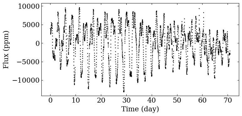
t, s0, dt = sp.load_k2_example ()
fig, ax = plt.subplots (1, 1, figsize=(8,4))

ax.scatter (t[s0!=0]-t[0], s0[s0!=0], color='black',
            marker='o', s=1)

ax.set_xlabel ('Time (day)')
ax.set_ylabel ('Flux (ppm)')

fig.tight_layout ()

plt.savefig ('figures/k2_lc.png', dpi=300)
pcutoff = 60
pthresh = 60
K2: Rotation period analysis#
In the next step, we compute the ACF and the WPS. We also analyse the characteristic periodicities obtained from the function, considering only periods below \(P_\mathrm{cutoff}\).
p_acf, acf = sp.compute_acf (s0, dt, normalise=True)
(_, _, _, _,
prots, hacf, gacf,
acf_smooth) = sp.find_period_acf (p_acf, acf, pcutoff=pcutoff,
                                  return_smoothed_acf=True)
fig = sp.plot_acf (p_acf, acf, prot=prots,
                   acf_additional=acf_smooth,
                   color_additional="darkorange",
                   filename='figures/acf_k2.png')
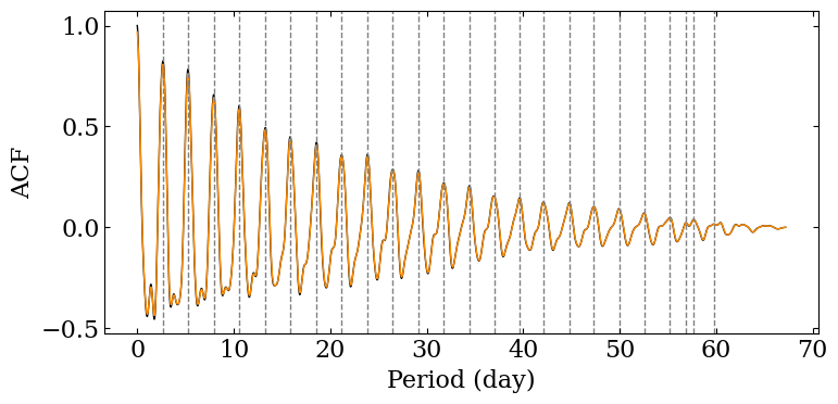
We can take a look at the values we have extracted from the ACF. Most
often, the rotation period can be linked to the first value of the
prots array.
prots[0], hacf[0], gacf[0]
(2.6765510971308686, 1.219105626528322, 0.8085280511689089)
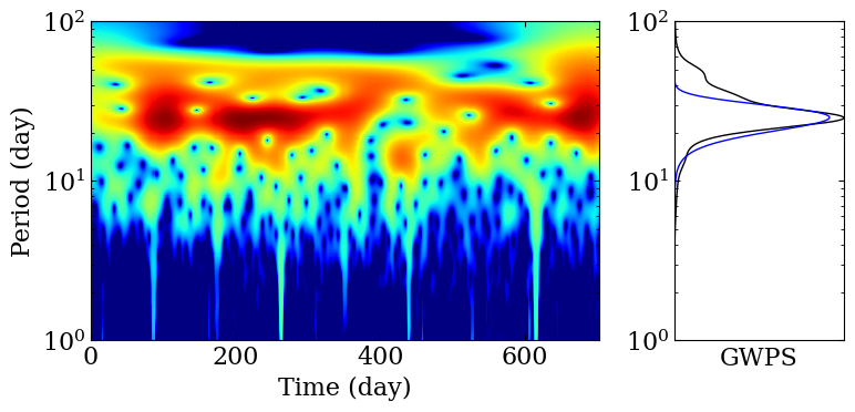
We now turn to the wavelet analysis
(periods, wps, gwps, _, _) = sp.compute_wps(s0, dt*86400, normalise=True)
(prot_ps, E_prot_ps,
 param_gauss) = sp.compute_prot_err_gaussian_fit (periods, gwps, n_profile=1)
fig = sp.plot_wps(t-t[0], periods, wps, gwps,
                  shading='auto', color_coi='darkgrey',
                  ylogscale=True, lw=1, normscale='log',
                  filename='figures/wps_k2.png', dpi=300,
                  figsize=(8,4), ylim=(1, 100),
                  show_contour=False,
                  param_gauss=param_gauss)

Let’s take a look at the result of the fit performed on the GPWS !
prot_ps, E_prot_ps
(2.6075837141864864, 0.3868209325802026)
Note that, due to the short length of this light curve, we do not show for this first case the analysis of long term modulations.
PLATO simulation: Preprocessing#
This first part include preprocessing tasks that are not actually included in MSAP4-02 but are useful for the subsequent analysis.
filename = sp.get_target_filename (plato_sim_dataset,
                                   '040', filetype='csv')
t, s0, dt = sp.load_resource (filename)
t, s0, dt = sp.rebin (t, 12), sp.rebin (s0, 12), dt*12
fig, ax = plt.subplots (1, 1, figsize=(8,4))

ax.scatter (t[s0!=0]-t[0], s0[s0!=0], color='black',
            marker='o', s=1)

ax.set_xlabel ('Time (day)')
ax.set_ylabel ('Flux (ppm)')

fig.tight_layout ()


plt.savefig ('figures/plato_lc.png', dpi=300)

s = sp.preprocess (t, s0, cut=60)
pcutoff = 60
pthresh = 60
PLATO simulation: Rotation period analysis#
This first part include preprocessing task that are not actually included in MSAP4-02 but are useful for the subsequent analysis.
fig, ax = plt.subplots (1, 1, figsize=(8,4))

ax.scatter (t[s!=0]-t[0], s[s!=0], color='black',
            marker='o', s=1)

ax.set_xlabel ('Time (day)')
ax.set_ylabel ('Flux (ppm)')

fig.tight_layout ()

plt.savefig ('figures/plato_lc_filtered.png', dpi=300)

p_acf, acf = sp.compute_acf (s, dt, normalise=True)
(_, _, _, _,
 prots, hacf, gacf,
 acf_smooth) = sp.find_period_acf (p_acf, acf, pcutoff=pcutoff,
                                   return_smoothed_acf=True)
fig = sp.plot_acf (p_acf, acf, prot=prots,
                   acf_additional=acf_smooth,
                   color_additional="darkorange",
                   filename='figures/acf_plato_short.png')

(periods, wps, gwps, _, _) = sp.compute_wps(s, dt*86400, normalise=True)
(prot_ps, E_prot_ps,
 param_gauss) = sp.compute_prot_err_gaussian_fit (periods, gwps, n_profile=1)
fig = sp.plot_wps(t-t[0], periods, wps, gwps,
                  shading='auto', color_coi='darkgrey',
                  ylogscale=True, lw=1, normscale='log',
                  filename='figures/wps_plato.png', dpi=300,
                  figsize=(8,4), ylim=(1, 100),
                  show_contour=False,
                  param_gauss=param_gauss)
Let’s take a look at the result of the fit performed on the GPWS !
PLATO simulation: Long term modulation analysis#
This time, we do not consider filtered out the data in order to consider long term modulations. We put a period threshold at 60 days to consider only long period in the postprocessing of our analysis. In the figure below, note that a Gaussian smoothing window is applied before looking for local maxima, shown in orange in the figure below.
s0 = sp.preprocess (t, s0, cut=60, desired=[1,1,0,0])
p_acf, acf = sp.compute_acf (s0, dt, normalise=True, pthresh=pthresh,
                            use_scipy_correlate=True, verbose=True)
(_, hacf, gacf, _,
pmods, hacf, gacf, acf_smooth) = sp.find_period_acf (p_acf, acf, pthresh=pthresh,
                                                     return_smoothed_acf=True)
fig = sp.plot_acf (p_acf, acf, prot=pmods,
                   acf_additional=acf_smooth,
                   color_additional="darkorange",
                   filename="figures/acf_plato_long.png")
