An example analysis framework#

This notebook provide an example of the analysis performed by the PLATO MSAP4-03 submodules: results from Lomb-Scargle periodogram, autocorrelation functions and composite spectrum are used to produce a set of features exploited by an existing instance of ROOSTER to return the final rotation period of the analysed target. You will find that what is done here is very similar to the ROOSTER tutorial notebook (rooster_training_framework, you should run it before doing this tutorial), the only big difference is actually that we will use here a pre-trained ROOSTER instance !

Here, the MSAP4-01A and MSAP4-02 steps required to feed MSAP4-03 are included in order to be able to run this notebook independently from the MSAP4-01A and MSAP4-02 notebooks.

Note that, due its significant computing time, the MSAP4-01B component dedicated to background analysis is executed independently in another notebook.

Note: This notebook has been designed for the purpose of scientific justification of MSAP4-03. The notebook illustrated the precise flowchart envisaged for MSAP4-03 is cs_rooster_sph_analysis.ipynb

import star_privateer as sp

sp.__version__

'1.1.1'

A simple example#

import os, pathos
from tqdm import tqdm
import numpy as np
import matplotlib.pyplot as plt

if not os.path.exists ('stellar_analysis_features') :
    os.mkdir ('stellar_analysis_features')

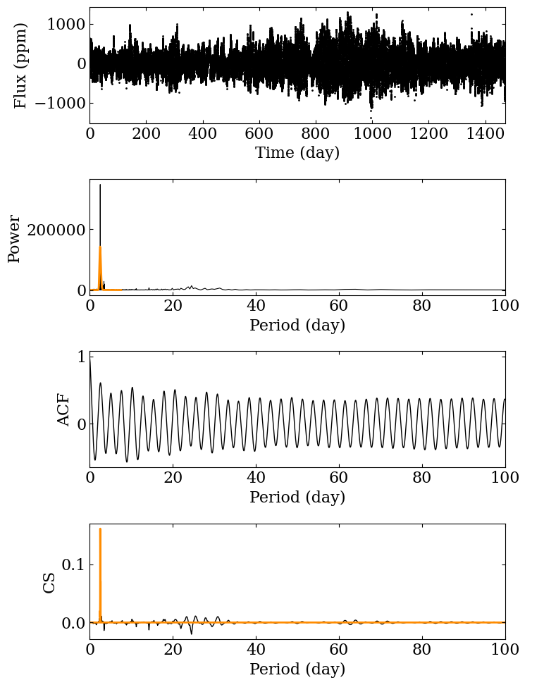
Our working case is KIC 3733735, a well-known Kepler fast rotating star.

filename = sp.get_target_filename (sp.timeseries, '003733735')
t, s, dt = sp.load_resource (filename)

The first thing we have to do is run the analysis pipeline. In particular, we can take a look at the plots made from the different analysis methods.

(p_ps, p_acf, ps, acf,
 cs, features, feature_names, _) = sp.analysis_pipeline (t, s, pmin=0.1, pmax=60, figsize=(8,10),
                                                            wavelet_analysis=False, plot=True,
                                                            filename='stellar_analysis_features/003733735.png',
                                                        )

../../_images/stellar_analysis_framework_8_0.png

We then save the results to a csv file:

fileout = 'stellar_analysis_features/003733735.csv'
df = sp.save_features (fileout, 3733735, features, feature_names)

As in the previous tutorial, let’s build a feature catalog. This is actually not required here because we are analysing only one star, but this step allows to ROOSTER-analyse several stars together with a simple framework.

df = sp.build_catalog_features ('stellar_analysis_features')

Then, let’s load the ROOSTER instance that we have trained in the previous tutorial:

chicken = sp.load_rooster_instance (filename='rooster_instances/rooster_tutorial')

As previously, let’s split the DataFrame into ROOSTER required inputs:

(target_id, p_candidates,
 e_p_candidates, E_p_candidates,
 features, feature_names) = sp.create_rooster_feature_inputs (df, return_err=True)

Here, we can see that there is actually (almost) nothing to do, as the three methods have yielded the same \(P_\mathrm{rot}\) estimate. However, we need ROOSTER to provide us with the rotation score of the target. ROOSTER will also select one of the three p_candidates as the final estimate for our target.

p_candidates

array([[2.53459872, 2.63594132, 2.56168138]])

The analyseSet function implemented in ROOSTER allows to analyse the features we extracted with the analysis pipeline. By providing feature_names, we ensure that ROOSTER was trained with the same features that those we extracted.

rotation_score, prot, e_p, E_p = chicken.analyseSet (features, p_candidates, e_p_err=e_p_candidates,
                                                     E_p_err=E_p_candidates, feature_names=feature_names)

We finally get the rotation score and the final \(P_\mathrm{rot}\). A rotation score above 0.5 means that the ROOSTER analysis favours a detection of stellar surface rotation signal.

rotation_score, prot, e_p, E_p

(array([0.78]), array([2.53459872]), array([0.21810524]), array([0.2634447]))

Analysing a PLATO simulated light curves dataset#

In order to illustrate the pipeline features described above, we can apply the pipeline to a larger dataset of 255 PLATO simulated light curves in order to check what we recover.

import plato_msap4_demonstrator_datasets.plato_sim_dataset as plato_sim_dataset

if not os.path.exists ('plato_sim_features') :
    os.mkdir ('plato_sim_features')

list_id = sp.get_list_targets (plato_sim_dataset)

Just as in the ROOSTER tutorial, we define a dedicated wrapper to analyse several light curves in parallel and avoid any memory leakage. Note than, we apply a 60-day high-pass finite impulse response filter to the simulated light curves (preprocess) function in order to remove low-frequency systematics while preserving at most the signature of stellar surface rotation in the data.

def analysis_wrapper (star_id) :
    """
    Analysis wrapper to speed computation
    by parallelising process and control
    memory usage.
    """
    star_id = str (star_id).zfill (3)
    fileout = 'plato_sim_features/{}.csv'.format(star_id)
    fileplot = 'plato_sim_features/{}.png'.format(star_id)
    filename = sp.get_target_filename (plato_sim_dataset, star_id, filetype='csv')
    if not os.path.exists (fileout) :
        t, s, dt = sp.load_resource (filename)
        s = sp.preprocess (t, s, cut=60)
        (p_ps, p_acf,
         ps, acf,
         cs, features,
         feature_names, fig) = sp.analysis_pipeline (t, s, pmin=0.1, pmax=60, plot=True,
                                                     wavelet_analysis=False, filename=fileplot,
                                                     figsize=(10,16), lw=1, dpi=300)
        df = sp.save_features (fileout, star_id, features, feature_names)
        plt.close ("all")

Let’s run the process pool:

process_pool = pathos.pools._ProcessPool (processes=4,
                                          maxtasksperchild=10)
with process_pool as p :
    list (tqdm (p.imap (analysis_wrapper,
                        list_id,
                        ),
                total=len (list_id))
          )
    p.close ()

100%|█████████████████████████████████████████████████████████████████████████████████████████████████████████████████████████| 255/255 [00:00<00:00, 843.21it/s]

We can now analyse the obtained features with ROOSTER to provide our final results.

df = sp.build_catalog_features ('plato_sim_features')
df

	prot_ps	prot_acf	prot_cs	e_prot_ps	E_prot_ps	e_prot_acf	E_prot_acf	e_prot_cs	E_prot_cs	sph_ps	sph_acf	sph_cs	h_ps	fa_prob_ps	hacf	gacf	hcs
target_id
0	42.955113	36.201157	43.493698	5.139282	6.755867	-1.0	-1.0	1.911796	1.911796	809.302045	770.019836	804.306555	4.573669e+06	0.0	0.522076	0.174793	0.804396
1	33.388871	32.603958	33.124768	7.850812	14.820267	-1.0	-1.0	5.027412	5.027412	197.317073	196.573468	196.860684	5.452245e+03	0.0	0.095639	0.045796	0.527596
2	17.529157	18.062384	17.308610	1.997207	2.586628	-1.0	-1.0	0.424356	0.424356	131.463440	132.741191	131.613358	9.626133e+03	0.0	0.226074	0.162293	0.137714
3	21.247463	20.791534	20.918945	2.308992	2.950196	-1.0	-1.0	0.729080	0.729080	108.132491	108.613715	108.524835	1.468874e+04	0.0	0.316458	0.308489	0.075097
4	28.636742	28.770649	29.353447	3.606657	4.821026	-1.0	-1.0	1.331297	1.331297	156.739595	156.556259	156.091130	8.556843e+02	0.0	0.021029	0.021854	0.433539
...	...	...	...	...	...	...	...	...	...	...	...	...	...	...	...	...	...
250	31.871195	29.319257	31.239800	9.996470	26.822076	-1.0	-1.0	4.055894	4.055894	213.718124	204.408037	215.372660	4.368693e+04	0.0	0.832173	0.428776	0.880686
251	20.214171	19.027656	20.212371	1.917448	2.366382	-1.0	-1.0	1.729649	1.729649	187.913408	178.586179	187.910206	8.072857e+04	0.0	0.688937	0.313818	0.835033
252	36.903489	37.805314	36.899833	5.608447	8.057559	-1.0	-1.0	5.558169	5.558169	1488.425513	1505.598715	1488.392507	8.011975e+06	0.0	1.508467	0.751838	0.976312
253	17.182045	17.395722	17.517652	2.098990	2.777632	-1.0	-1.0	2.245630	2.245630	164.770235	164.282166	164.016051	1.954305e+04	0.0	0.613475	0.262470	0.091111
254	18.950440	18.659603	18.951406	1.989637	2.518474	-1.0	-1.0	0.592259	0.592259	1210.035639	1216.557654	1209.993163	7.215866e+06	0.0	0.813409	0.298095	0.997597

255 rows × 17 columns

(target_id, p_candidates,
 e_p_candidates, E_p_candidates,
 features, feature_names) = sp.create_rooster_feature_inputs (df, return_err=True)
rotation_score, prot, e_p, E_p = chicken.analyseSet (features, p_candidates, e_p_err=e_p_candidates,
                                                     E_p_err=E_p_candidates, feature_names=feature_names)

Next, let’s load the reference catalog for these simulated light curves in order to compare the results from our pipeline with what was injected in the data.

prot_ref = sp.get_prot_ref (target_id, catalog='plato-sim')
cond_0 = (rotation_score>0.5)
cond_1 = (np.abs (prot - prot_ref) < 0.1 * prot_ref)
cond_2 = (np.abs (prot - prot_ref) < 0.1 * prot_ref) & (rotation_score>0.5)
score_0 = target_id[cond_0].size / target_id.size
score_1 = target_id[cond_1].size / target_id.size
score_2 = target_id[cond_2].size / target_id.size
score_0, score_1, score_2

(0.9450980392156862, 0.615686274509804, 0.596078431372549)

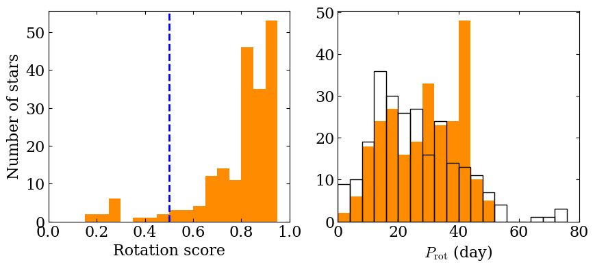
The score computed here means that we were able to successfully detect a rotation signal and recover the correct rotation period for about 61% of the stars in the sample. We can take a look at histograms to check the rotation score of our population and to compare the input rotation periods distribution to the one we recover.

fig, (ax1, ax2) = plt.subplots (1, 2, figsize=(10, 4))

bins = np.linspace (0, 1, 20, endpoint=False)
ax1.hist (rotation_score, bins=bins, color='darkorange')
ax1.axvline (0.5, ls='--', color='blue', lw=2)
bins = np.linspace (0, 80, 20, endpoint=False)
ax2.hist (prot, bins=bins, color='darkorange')
ax2.hist (prot_ref, bins=bins, facecolor='none',
         edgecolor='black', label='Ref')

ax1.set_ylabel (r'Number of stars')
ax1.set_xlabel (r'Rotation score')
ax2.set_xlabel (r'$P_\mathrm{rot}$ (day)')

ax1.set_xlim (0, 1)
ax2.set_xlim (0, 80)

(0.0, 80.0)

../../_images/stellar_analysis_framework_36_1.png

An example analysis framework

Contents

An example analysis framework#

A simple example#

Analysing a PLATO simulated light curves dataset#