ROOSTER training framework (MSAP4-03)#

This notebook provide an example of the analysis of a set of stars with catalog-existing reference \(P_\mathrm{rot}\), and use the set to train an instance of ROOSTER.

First we need to import the demonstrator module and the auxiliary module containing the dataset we are going to work with.

Note: This notebook has been designed for the purpose of scientific justification of PLATO MSAP4-03. The notebook illustrated the precise flowchart envisaged for PLATO MSAP4-03 is cs_rooster_sph_analysis.ipynb

import star_privateer as sp
import plato_msap4_demonstrator_datasets.kepler_dataset as kepler_dataset

sp.__version__

'1.1.2'

We also need to import some other modules to run the notebook and to check that the outputs directory that we need exist. In addition to star_privateer requirements, you should make sure that the `pathos module <https://pathos.readthedocs.io/en/latest/index.html>`__ is installed in order to run the analysis in parallel.

import os, pathos
import numpy as np
import matplotlib.pyplot as plt
from tqdm import tqdm

if not os.path.exists ('rooster_training_features') :
    os.mkdir ('rooster_training_features')
if not os.path.exists ('rooster_instances') :
    os.mkdir ('rooster_instances')

Running the analysis pipeline#

We are going to work with a sample of 1991 Kepler stars analysed by Santos et al. (2019, 2021). The light curves have been calibrated with the KEPSEISMIC method (see García et al. 2011, 2014), and all of them have been filtered with a 55-day high-pass filter. We can get the identifiers of the stars in the dataset with the following instruction:

list_kic = sp.get_list_targets (kepler_dataset)

The next step is to run the analysis pipeline on every light curve in the dataset. The analysis pipeline in its default behaviour will compute the Lomb-Scargle periodogram (LSP) of the light curve as well as its auto-correlation function (ACF). ACF and LSP will then be used to compute a composite spectrum (CS), obtained by multiplying one by another. The feature computed for each stars are stored in a dedicated csv file identified by the star identifier (in this case, the KIC of the star). We are going to parallelise the analysis process with pathos in order to gain some computation time and control memory leakages that could arise from calling analysis_pipeline in a loop.

def analysis_wrapper (kic) :
    """
    Analysis wrapper to speed computation
    by parallelising process and control
    memory usage.
    """
    str_kic = str (kic).zfill (9)
    filename = sp.get_target_filename (kepler_dataset, str_kic)
    fileout = 'rooster_training_features/{}.csv'.format(str_kic)
    fileplot = 'rooster_training_features/{}.png'.format(str_kic)
    if not os.path.exists (fileout) :
        t, s, dt = sp.load_resource (filename)
        (p_ps, p_acf,
         ps, acf,
         cs, features,
         feature_names,
         fig) = sp.analysis_pipeline (t, s, pmin=0.1, pmax=60,
                                      wavelet_analysis=False, plot=True,
                                      filename=fileplot, figsize=(10,16),
                                      lw=1, dpi=300, pfa_threshold=1e-6)
        df = sp.save_features (fileout, kic, features, feature_names)
        plt.close ("all")

Now that are wrapper function is defined, we just create a ProcessPool that we run with imap:

Note: by default imap, on the contrary to map, is a non-blocking process. Nevertheless, in order to display a progress bar with tqdm we need to use it, and the list encapsulation is there to ensure the process is blocking.

process_pool = pathos.pools._ProcessPool (processes=4,
                                          maxtasksperchild=10)
with process_pool as p :
    list (tqdm (p.imap (analysis_wrapper,
                        list_kic,
                        ),
                total=len (list_kic))
          )
    p.close ()

100%|██████████████████████████████████████████████████████████████████████████████████████████████████████████████████████| 1991/1991 [00:02<00:00, 682.41it/s]

After running the analysis pipeline, it is possible to concatenate the feature obtained for each star into one big DataFrame.

df = sp.build_catalog_features ('rooster_training_features')

This is typically what the DataFrame is going to look like:

df

	prot_ps	prot_acf	prot_cs	e_prot_ps	E_prot_ps	e_prot_acf	E_prot_acf	e_prot_cs	E_prot_cs	sph_ps	sph_acf	sph_cs	e_sph_ps	e_sph_acf	e_sph_cs	h_ps	fa_prob_ps	hacf	gacf	hcs
target_id
891901	5.583862	51.574947	5.641521	0.451109	0.538044	-1.0	-1.0	0.013094	0.013094	621.412430	773.889578	620.957800	245.146024	101.483976	224.734810	388.571741	1.759694e-169	0.277619	0.109637	0.012586
1162339	0.493096	-1.000000	0.976043	0.000351	0.000351	-1.0	-1.0	0.011880	0.011880	462.872324	-1.000000	578.779362	359.874252	-1.000000	430.008329	371.694864	3.758129e-162	-1.000000	-1.000000	0.040937
1163248	5.791226	59.625771	3.136216	0.005828	0.005840	-1.0	-1.0	0.166361	0.166361	443.149604	541.775945	346.123281	163.047747	41.778081	98.225272	20.010528	2.039567e-09	0.271948	0.135494	0.580406
1164583	50.378386	43.891695	1.465304	-1.000000	-1.000000	-1.0	-1.0	0.579764	0.579764	1650.421415	1642.510883	667.192946	484.602802	463.437724	370.658390	12.330474	4.415127e-06	0.635193	0.317102	1.218906
1433067	47.138724	-1.000000	30.768920	0.047102	0.047197	-1.0	-1.0	2.141848	2.141848	1197.078140	-1.000000	1142.311679	306.901676	-1.000000	360.490565	20.918206	8.228836e-10	-1.000000	-1.000000	0.218161
...	...	...	...	...	...	...	...	...	...	...	...	...	...	...	...	...	...	...	...	...
12647815	10.435607	10.421169	10.439005	0.010425	0.010446	-1.0	-1.0	0.052430	0.052430	4727.467867	4731.485721	4725.580181	1638.084281	1651.040028	1635.984428	321.261367	3.005808e-140	0.993603	0.606440	0.928269
12737258	40.589407	-1.000000	40.522208	0.040555	0.040637	-1.0	-1.0	0.877765	0.877765	2135.275789	-1.000000	2138.867175	598.419531	-1.000000	592.453395	39.599624	6.340181e-18	-1.000000	-1.000000	0.158801
12784167	0.612374	12.709734	18.235136	0.000006	0.000006	-1.0	-1.0	0.197108	0.197108	346.990379	615.325577	631.680180	55.723119	142.765932	128.610360	103.591522	1.025118e-45	0.000056	0.082313	0.722011
12834290	52.678504	57.295905	3.254078	0.052611	0.052717	-1.0	-1.0	0.124075	0.124075	528.655933	527.046251	361.159430	89.142743	76.276120	70.506151	15.638527	1.615377e-07	0.197379	0.076179	0.160712
12834663	0.339495	-1.000000	1.628611	-1.000000	-1.000000	-1.0	-1.0	0.041504	0.041504	712.198133	-1.000000	787.582801	86.012201	-1.000000	160.792154	6.598372	1.362585e-03	-1.000000	-1.000000	0.207903

1991 rows × 20 columns

df.to_csv ("training_features.csv")

Training and testing ROOSTER#

Now that we have analysed a large sample of stars, we are able to use it to train the random forest ROOSTER methodology (see Breton et al. 2021). First, let’s (arbitrarily) divide our DataFrame into a training set and a test set.

df_train = df.sample (n=df.index.size//2, random_state=49458493)
df_test = df.loc[np.setdiff1d (df.index, df_train.index)]

The DataFrames let us obtain all the input we require to train and test ROOSTER:

(training_id, training_p_candidates,
 training_features, feature_names) = sp.create_rooster_feature_inputs (df_train)
(test_id, test_p_candidates,
 test_features, test_feature_names) = sp.create_rooster_feature_inputs (df_test)

Now, let’s instantiate a new ROOSTER object. The main attributes of ROOSTER are its two random forest classifiers, RotClass and PeriodSel. The properties of these classifiers can be specified by the user by passing the optional arguments of sklearn.ensemble.RandomForestClassifier to the created ROOSTER instance.

feature_names

Index(['E_prot_acf', 'E_prot_cs', 'E_prot_ps', 'e_prot_acf', 'e_prot_cs',
       'e_prot_ps', 'e_sph_acf', 'e_sph_cs', 'e_sph_ps', 'fa_prob_ps', 'gacf',
       'h_ps', 'hacf', 'hcs', 'prot_acf', 'prot_cs', 'prot_ps', 'sph_acf',
       'sph_cs', 'sph_ps'],
      dtype='object')

seed = 104359357
chicken = sp.ROOSTER (n_estimators=100, random_state=np.random.RandomState (seed=seed))
chicken.RotClass, chicken.PeriodSel

(RandomForestClassifier(random_state=RandomState(MT19937) at 0x133CCD040),
 RandomForestClassifier(random_state=RandomState(MT19937) at 0x133CCD040))

The training is performed as follows:

chicken.train (training_id, training_p_candidates,
               training_features, feature_names=feature_names,
               catalog='santos-19-21', verbose=True)

Training RotClass with 392 stars with detected rotation and 493 without detected rotation.
Training PeriodSel with 392 stars.

Once properly trained, ROOSTER performances can be assessed with our test set:

results = chicken.test (test_id, test_p_candidates, test_features,
                        feature_names=test_feature_names,
                        catalog='santos-19-21', verbose=True)

Testing RotClass with 380 stars with detected rotation and 502 without detected rotation.
Testing PeriodSel with 380 stars.

The score obtained during the test set can be accessed through the getScore function, as well as the number of elements used for the training and the test steps.

chicken.getScore ()

(0.9263038548752834, 0.9315789473684211)

chicken.getNumberEltTrain ()

(885, 392)

chicken.getNumberEltTest ()

(882, 380)

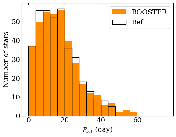
The \(P_\mathrm{rot}\) computed by ROOSTER for the test set are returned when calling the function and it can be interesting to plot the distribution to compare it to the reference catalog values.

prot_rooster = results[3]
prot_ref = sp.get_prot_ref (results[2], catalog='santos-19-21')

Let’s take a look at the corresponding histogram

fig, ax = plt.subplots (1, 1)

bins = np.linspace (0, 80, 20, endpoint=False)

ax.hist (prot_rooster, bins=bins, color='darkorange', label='ROOSTER')
ax.hist (prot_ref, bins=bins, facecolor='none',
        edgecolor='black', label='Ref')

ax.set_xlabel (r'$P_\mathrm{rot}$ (day)')
ax.set_ylabel (r'Number of stars')

ax.legend ()

<matplotlib.legend.Legend at 0x1335b7af0>

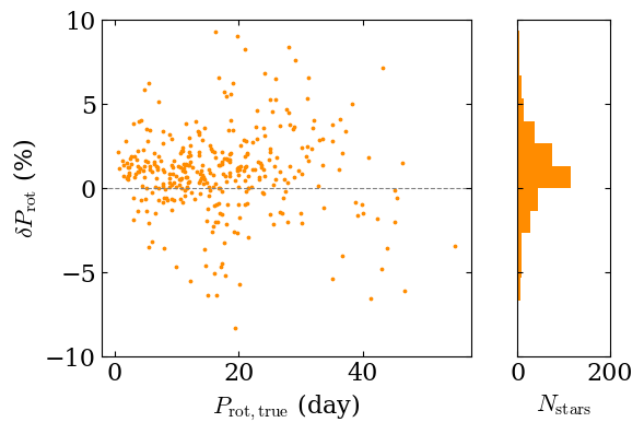
../../_images/rooster_training_framework_35_1.png

It can also be instructive to compare directly the ROOSTER results to the reference values.

fig, (ax, ax0) = plt.subplots (1, 2, figsize=(6, 4),
                               width_ratios=[0.8, 0.2],
                               sharey=True)

ax.scatter (prot_ref, (prot_rooster - prot_ref) / prot_ref * 100,
            color='darkorange', s=3, marker="o")

ax0.hist ((prot_rooster - prot_ref) / prot_ref * 100,
          bins=np.linspace (-20, 20, 31), orientation="horizontal",
          color="darkorange")

ax.set_xlabel (r'$P_\mathrm{rot, true}$ (day)')
ax.set_ylabel (r"$\delta P_\mathrm{rot}$ (%)")

ax.axhline (0, ls="--", color="grey")

ax.set_ylim (-10, 10)

ax0.set_xlim (0, 200)
ax0.set_xlabel (r"$N_\mathrm{stars}$")

Text(0.5, 0, '$N_\mathrm{stars}$')

../../_images/rooster_training_framework_37_1.png

Finally, let’s save our trained ROOSTER instance to be able to use it again later (for example in the next tutorial notebook !)

chicken.save ('rooster_instances/rooster_tutorial')

ROOSTER training framework (MSAP4-03)

Contents

ROOSTER training framework (MSAP4-03)#

Running the analysis pipeline#

Training and testing ROOSTER#